Conditional Formatting in Google Sheets: This Week, Next Week, Last Week
The Very Basics of Conditional Formatting
Conditional formatting is used when you want to apply styles to a large number of cells using data within cells to determine how a cell is formatted. Maybe you want to draw attention to dates that are getting near, such as a deadline, or maybe you want to color a range of cells based on a "high-priority" label or something similar.
Using conditional formatting is fairly simple for most applications. Just select a range of cells (including whole columns or groups of columns), then choose Format > Conditional formatting from the menu.
From there, you can use any of the pre-defined custom formatting options provided by Google, or you can write your own custom formulas for more complex interactions.
We've covered a lot about using custom formulas for conditional formatting in Google Sheets, especially color-coding cells based on the date. Now let's look at how to color-code cells based on whether a date contained in a cell falls in this week, next week, last week or any other week.
For this tutorial, we'll shade a cell green if the date in that cell is in this week, yellow if it's next week and red if it's last week. For this example, we'll put our date fields in column B and also color-code those date fields in column B. Note that the dates can be in any column you choose, and you can color code any column based on the date in the same or any other column.
So the basic formula we want to create will color a cell in column B if a date in column B falls in the same week as today's date.
Long Story Short
For those of you who aren't interested in the whys or hows, here are the formulas you can plug into your Custom Formula field in the Conditional Formatting dialog.
For a date that occurs within the current week, assuming the week starts on a Sunday and ends on a Saturday:
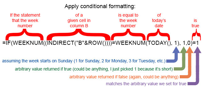
=IF(WEEKNUM((INDIRECT("B"&ROW())))=WEEKNUM(TODAY(), 1), 1,0)=1
For a date that occurs next week:
=if(WEEKNUM((INDIRECT("B"&ROW())))=WEEKNUM((TODAY()+7), 1), 1,0)=1
For a date that occurred last week:
=if(WEEKNUM((INDIRECT("B"&ROW())))=WEEKNUM((TODAY()-7), 1), 1,0)=1
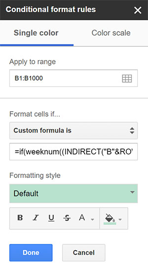
Paste the formula into the Conditional
formatting pane as seen above.
Long Story Long
For those who want to understand how this works so you can extrapolate other uses, here's what all of that means.
To make this work, we need a few operators:
So, looking at the formula for this week, we can break it down as follows:
So how would you extrapolate from that to compare a date to next week instead of this week?
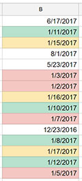
The formatted cells.
The portion "WEEKNUM(TODAY(), 1)" means the week number of today's date, given that the week starts on Sunday. So next week would simply be the date seven days later, which would be written: "WEEKNUM((TODAY()+7), 1)," with an extra set of parentheses around (TODAY()+7).
What about last week then? You guessed it: "WEEKNUM((TODAY()-7), 1)."
And you can extrapolate from there the method for formatting a date with any given week number.
You can find more tutorials on conditional formatting and the use of custom formulas on our Google G Suite tutorial archive.