Learn how to use Google Classroom's assignments feature to create and manage group projects for students.
We've covered a lot about using custom formulas for conditional formatting in Google Sheets, especially color-coding cells based on the date. Now let's look at how to color-code cells based on whether a date contained in a cell falls in this week, next week, last week or any other week.
Common wisdom says you just can't apply conditional formatting in a Google Apps spreadsheet using data from a different sheet. But here at THE Journal, we laugh in the face of wisdom, common or otherwise. But is such jocularity is justified? Read on.

This week's tutorial covers a number functions in Google's Spreadsheet app, Google Sheets. Here we take a practical look at using weekdays in calculations, introduce "if" statements and learn how to refer dynamically to the contents of a current cell.

Here's a quick and dirty formula you can use in Google Sheets to get a running count of cells that contain any value (numbers, dates, text, links, etc.).

This question comes up often in user forums: How do I extract a piece of information from one column and put that extracted information into another? For example, if I have a URL in one column, can I extract the date from that URL and put it in my date column so I don't have to the the date manually?

In our first tutorial on Google Sheets, we looked at extending the software's default conditional formatting options through the use of formulas. That solution is good for a limited range of dates, but it might get cumbersome in spreadsheets that span longer periods, since each possible date requires a unique formula.

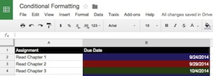
Google Sheets, the spreadsheet tool that's part of the Google Apps productivity suite, lets users format cells based on certain conditions, including the date contained in a cell and how far away that date is from the present. But the options available through the Conditional Formatting dialog are limited. Here's a way around those limitations.